Predict disease classes using genetic microarray data
Objective
The purpose of this article is to show how to develop a method that uses genetic data for disease classification. Data is extracted from a DNA microarray which measures the expression levels of large numbers of genes simultaneously.
Samples in the datasets represent patients. For each patient 7070 genes expressions (values) are measured in order to classify the patient’s disease into one of the following cases: EPD, JPA, MED, MGL, RHB.
Data
Gene data is in genes-in-rows format, comma-separated values. There are following 3 files on my GitHub:
- Training dataset: pp5i_train.gr.csv
- Training data classes: pp5i_train_class.txt
- Test dataset: pp5i_test.gr.csv
Instructions
Training data: file pp5i_train.gr.csv, with 7070 genes for 69 samples. A separate file pp5i_train_class.txt has classes for each sample, in the order corresponding to the order of samples in pp5i_train.gr.cdv.
Test data: file pp5i_test.gr.csv, with 23 unlabelled samples and same genes. Assume that the class distribution is similar.
The goal is to learn the best model from the training data and use it to predict the label (class) for each sample in test data. Randomization experiments showed that one can get about 10-12 (from 23) correct answers with random guessing.
Hints
Be sure that don’t use the sample number as one of the predictors. Training data is ordered by class, so sample number will be appear to be a good predictor on cross-validation, but it will not work on the test data.
One of the MED samples in the training data is very likely misclassified (by a human). So the best result expected to get on cross-validation is one error (on a MED sample) out of 69. However, this doesn’t affect accuracy on the test set.
Here I use Python and its libraries. The following steps are one way of finding the best model.
Steps
Read data
import pandas as pd

train_data = pd.read_csv('pp5i_train.gr.csv', index_col=0)
test_data = pd.read_csv('pp5i_test.gr.csv', index_col=0)
train_class = pd.read_csv('pp5i_train_class.txt')
print(train_class['Class'].value_counts())
The class distribution as follows:
MED    39
EPD    10
MGL     7
RHB     7
JPA     6
Name: Class, dtype: int64
Data Cleaning
Threshold both train and test data to a minimum value of 20, maximum of 16,000. Remove null values.
import numpy as np

train_data[(train_data < 20) | (train_data > 16000)] = np.nan
test_data[(test_data < 20) | (test_data > 16000)] = np.nan

train_data_clean = train_data[(~train_data.isnull().any(1)) & (~test_data.isnull().any(1))]
test_data_clean = test_data[(~train_data.isnull().any(1)) & (~test_data.isnull().any(1))]
Select top genes by class
- Remove from train data genes with fold differences across samples less than 2. Fold difference is defined as a ratio between maximum and minimum values (Max/Min) for a given data set.
train_data_fold = train_data_clean[train_data_clean.apply(lambda x: x.max()/x.min() > 2, axis=1)]
- For each class, generate subsets with top 2, 4, 6, 8, 10, 12, 15, 20, 25, and 30 top genes with the highest absolute T-value. The Objective is to find for each class the set of best genes to discriminate it from the other classes.
from scipy import stats

classes = np.unique(train_class.values)

t_values = pd.DataFrame(index=train_data_fold.index.tolist())
for label in classes:
  for gene in train_data_fold.index.tolist():
    cur_samples = train_data_fold.loc[gene][np.ravel((train_class==label).values.tolist())]
    rest_samples = train_data_fold.loc[gene][np.ravel((train_class!=label).values.tolist())]
    t_values.loc[gene, label] = abs(stats.ttest_ind(cur_samples, rest_samples,
                                                    equal_var=False, nan_policy='raise')[0])
- For \(N = 2, 4, 6, 8, 10, 12, 15, 20, 25, 30\) combine top genes for each class into one file (removing duplicates, if any) and call the resulting file pp5i_train.topN.gr.csv. Add the class as the last column, remove sample no, transpose each file to “gene-in-columns” format.
N = [2,4,6,8,10,12,15,20,25,30]

for n in N:
  top_genes = set()
  for label in classes:
    top_genes.update(t_values.sort_values(label, ascending=False).head(n).index.tolist())
  pd.concat([train_data_fold.loc[list(top_genes), :].T.reset_index(drop=True), train_class],
            axis=1).to_csv('pp5i_train.top'+str(n)+'.gr.csv', index=False)
Find the best classifier/best gene set combination
Use following classifiers:
- Naïve Bayes
- Decision Tree
- K-NN
- Neural Network
- Random Forest
For each classifier, using default settings, measure classifier accuracy on the training set using previously generated files with top \(N = 2, 4, 6, 8, 10, 12, 15, 20, 25, 30\) genes.
Select the model and the gene set with the lowest cross-validation error. Cross-validation is the main tool to measure classification accuracy. In Scikit-learn, it shows how it can be calculated.
Once found the gene set with the lowest cross-validation error, vary 1-2 additional relevant parameters for each classifier to improve the accuracy.
Naïve Bayes
from sklearn.naive_bayes import GaussianNB
from sklearn.model_selection import cross_val_score

GNBclf = GaussianNB()

def search_gene(clf):
    best_score = 0
    accuracy = []
    for n in N:
        scores = cross_val_score(GNBclf, globals()['x_train%s'%n], globals()['y_train%s'%n], cv=5, n_jobs=-1)
        score = scores.mean()
        accuracy.append(score)
        print("N=%d accuracy: %0.2f (+/- %0.2f)" % (n, score, scores.std() * 2))
        best_n = n if score > best_score else best_n
        best_score = score if score > best_score else best_score
    return best_n, accuracy

best_n, scores = search_gene(GNBclf)
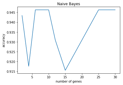
N=2 accuracy: 0.94 (+/- 0.11)
N=4 accuracy: 0.92 (+/- 0.14)
N=6 accuracy: 0.95 (+/- 0.10)
N=8 accuracy: 0.95 (+/- 0.10)
N=10 accuracy: 0.95 (+/- 0.10)
N=12 accuracy: 0.93 (+/- 0.08)
N=15 accuracy: 0.92 (+/- 0.11)
N=20 accuracy: 0.93 (+/- 0.08)
N=25 accuracy: 0.95 (+/- 0.10)
N=30 accuracy: 0.95 (+/- 0.10)
Next, try different types of naïve bayes:
from sklearn.naive_bayes import MultinomialNB, ComplementNB, BernoulliNB

MNBclf = MultinomialNB()
CNBclf = ComplementNB()
BNBclf = BernoulliNB()

for c in ['G', 'M', 'C', 'B']:
    scores = cross_val_score(globals()[c+'NBclf'], globals()['x_train%s' % best_n], globals()['y_train%s' % best_n], cv=5, n_jobs=-1)
    print("N=%d %sNBclf accuracy: %0.2f (+/- %0.2f)" % (best_n, c, scores.mean(), scores.std() * 2))
N=6 GNBclf accuracy: 0.95 (+/- 0.10)
N=6 MNBclf accuracy: 0.96 (+/- 0.11)
N=6 CNBclf accuracy: 0.86 (+/- 0.12)
N=6 BNBclf accuracy: 0.57 (+/- 0.09)
Decision Tree
from sklearn.tree import DecisionTreeClassifier

DTclf = DecisionTreeClassifier()

best_n, scores = search_gene(DTclf)
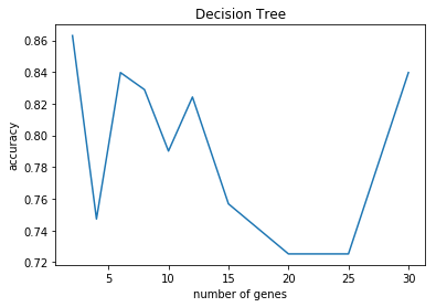
N=2 accuracy: 0.78 (+/- 0.31)
N=4 accuracy: 0.78 (+/- 0.20)
N=6 accuracy: 0.80 (+/- 0.29)
N=8 accuracy: 0.84 (+/- 0.31)
N=10 accuracy: 0.80 (+/- 0.29)
N=12 accuracy: 0.79 (+/- 0.21)
N=15 accuracy: 0.72 (+/- 0.35)
N=20 accuracy: 0.82 (+/- 0.27)
N=25 accuracy: 0.69 (+/- 0.37)
N=30 accuracy: 0.73 (+/- 0.29)
Then search for best parameters in decision tree model:
from sklearn.model_selection import GridSearchCV


params = {
    'max_depth': [30, 60, 90, None],
    'class_weight': ['balanced', None]
}

def print_results(results):
    print('Best Params: {}\n'.format(results.best_params_))
    means = results.cv_results_['mean_test_score']
    stds = results.cv_results_['std_test_score']
    for mean, std, params in zip(means, stds, results.cv_results_['params']):
        print('{} (+/-{}) for {}'.format(round(mean, 2), round(std * 2, 2), params))

def search_param(clf, params, n):
    cv = GridSearchCV(clf, params, cv=5, n_jobs=-1, iid=False)
    cv.fit(globals()['x_train%s' % n], globals()['y_train%s' % n])

    print('N=%s:' % n)
    print_results(cv)

search_param(DTclf, params, best_n)
N=8:
Best Params: {'class_weight': None, 'max_depth': 30}

0.81 (+/-0.19) for {'class_weight': 'balanced', 'max_depth': 30}
0.82 (+/-0.27) for {'class_weight': 'balanced', 'max_depth': 60}
0.81 (+/-0.19) for {'class_weight': 'balanced', 'max_depth': 90}
0.86 (+/-0.18) for {'class_weight': 'balanced', 'max_depth': None}
0.89 (+/-0.14) for {'class_weight': None, 'max_depth': 30}
0.78 (+/-0.23) for {'class_weight': None, 'max_depth': 60}
0.76 (+/-0.34) for {'class_weight': None, 'max_depth': 90}
0.77 (+/-0.26) for {'class_weight': None, 'max_depth': None}
K-NN
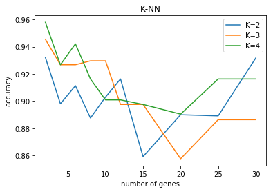
For K-NN, test accuracy with \(K = 2, 3, 4\).
from sklearn.neighbors import KNeighborsClassifier

KNNclf = KNeighborsClassifier(n_jobs=-1)

params = {
    'n_neighbors': [2, 3, 4]
}

best_score = 0
for n in N:
    cv = GridSearchCV(KNNclf, params, cv=5, n_jobs=-1, iid=False)
    cv.fit(globals()['x_train%s'%n], globals()['y_train%s'%n])
    score = max(cv.cv_results_['mean_test_score'])
    best_n = n if score > best_score else best_n
    best_K = cv.best_params_['n_neighbors'] if score > best_score else best_K
    best_score = score if score > best_score else best_score
    print('N=%s:'%n)
    print_results(cv)
N=2:
Best Params: {'n_neighbors': 4}

0.93 (+/-0.15) for {'n_neighbors': 2}
0.95 (+/-0.1) for {'n_neighbors': 3}
0.96 (+/-0.11) for {'n_neighbors': 4}
N=4:
Best Params: {'n_neighbors': 3}

0.9 (+/-0.07) for {'n_neighbors': 2}
0.93 (+/-0.02) for {'n_neighbors': 3}
0.93 (+/-0.02) for {'n_neighbors': 4}
N=6:
Best Params: {'n_neighbors': 4}

0.91 (+/-0.07) for {'n_neighbors': 2}
0.93 (+/-0.02) for {'n_neighbors': 3}
0.94 (+/-0.06) for {'n_neighbors': 4}
N=8:
Best Params: {'n_neighbors': 3}

0.89 (+/-0.14) for {'n_neighbors': 2}
0.93 (+/-0.08) for {'n_neighbors': 3}
0.92 (+/-0.09) for {'n_neighbors': 4}
N=10:
Best Params: {'n_neighbors': 3}

0.9 (+/-0.13) for {'n_neighbors': 2}
0.93 (+/-0.08) for {'n_neighbors': 3}
0.9 (+/-0.05) for {'n_neighbors': 4}
N=12:
Best Params: {'n_neighbors': 2}

0.92 (+/-0.09) for {'n_neighbors': 2}
0.9 (+/-0.08) for {'n_neighbors': 3}
0.9 (+/-0.05) for {'n_neighbors': 4}
N=15:
Best Params: {'n_neighbors': 3}

0.86 (+/-0.16) for {'n_neighbors': 2}
0.9 (+/-0.08) for {'n_neighbors': 3}
0.9 (+/-0.08) for {'n_neighbors': 4}
N=20:
Best Params: {'n_neighbors': 4}

0.89 (+/-0.2) for {'n_neighbors': 2}
0.86 (+/-0.07) for {'n_neighbors': 3}
0.89 (+/-0.15) for {'n_neighbors': 4}
N=25:
Best Params: {'n_neighbors': 4}

0.89 (+/-0.18) for {'n_neighbors': 2}
0.89 (+/-0.1) for {'n_neighbors': 3}
0.92 (+/-0.09) for {'n_neighbors': 4}
N=30:
Best Params: {'n_neighbors': 2}

0.93 (+/-0.12) for {'n_neighbors': 2}
0.89 (+/-0.1) for {'n_neighbors': 3}
0.92 (+/-0.09) for {'n_neighbors': 4}
KNN4clf = KNeighborsClassifier(n_neighbors=4, n_jobs=-1)

params = {
    'n_neighbors': [2, 3, 4],
    'weights' : ['uniform', 'distance']
}

search_param(KNN4clf, params, best_n)
N=2:
Best Params: {'n_neighbors': 4, 'weights': 'uniform'}

0.93 (+/-0.15) for {'n_neighbors': 2, 'weights': 'uniform'}
0.93 (+/-0.13) for {'n_neighbors': 2, 'weights': 'distance'}
0.95 (+/-0.1) for {'n_neighbors': 3, 'weights': 'uniform'}
0.95 (+/-0.1) for {'n_neighbors': 3, 'weights': 'distance'}
0.96 (+/-0.11) for {'n_neighbors': 4, 'weights': 'uniform'}
0.95 (+/-0.1) for {'n_neighbors': 4, 'weights': 'distance'}
Neural Network
from sklearn.neural_network import MLPClassifier

NNclf = MLPClassifier()
best_n, scores = search_gene(NNclf)
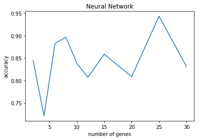
N=2 accuracy: 0.84 (+/- 0.27)
N=4 accuracy: 0.72 (+/- 0.43)
N=6 accuracy: 0.88 (+/- 0.18)
N=8 accuracy: 0.90 (+/- 0.13)
N=10 accuracy: 0.84 (+/- 0.17)
N=12 accuracy: 0.81 (+/- 0.27)
N=15 accuracy: 0.86 (+/- 0.19)
N=20 accuracy: 0.81 (+/- 0.23)
N=25 accuracy: 0.94 (+/- 0.06)
N=30 accuracy: 0.83 (+/- 0.11)
params = {
    'hidden_layer_sizes' : [(100,), (200,), (400,)],
    'activation' : ['identity', 'logistic', 'tanh', 'relu']
}

search_param(NNclf, params, best_n)
N=8:
Best Params: {'activation': 'logistic', 'hidden_layer_sizes': (200,)}

0.83 (+/-0.21) for {'activation': 'identity', 'hidden_layer_sizes': (100,)}
0.89 (+/-0.15) for {'activation': 'identity', 'hidden_layer_sizes': (200,)}
0.86 (+/-0.12) for {'activation': 'identity', 'hidden_layer_sizes': (400,)}
0.94 (+/-0.11) for {'activation': 'logistic', 'hidden_layer_sizes': (100,)}
0.97 (+/-0.06) for {'activation': 'logistic', 'hidden_layer_sizes': (200,)}
0.97 (+/-0.06) for {'activation': 'logistic', 'hidden_layer_sizes': (400,)}
0.91 (+/-0.13) for {'activation': 'tanh', 'hidden_layer_sizes': (100,)}
0.95 (+/-0.1) for {'activation': 'tanh', 'hidden_layer_sizes': (200,)}
0.97 (+/-0.07) for {'activation': 'tanh', 'hidden_layer_sizes': (400,)}
0.87 (+/-0.17) for {'activation': 'relu', 'hidden_layer_sizes': (100,)}
0.88 (+/-0.07) for {'activation': 'relu', 'hidden_layer_sizes': (200,)}
0.89 (+/-0.09) for {'activation': 'relu', 'hidden_layer_sizes': (400,)}
Random Forest
from sklearn.ensemble import RandomForestClassifier

RFclf = RandomForestClassifier(n_jobs=-1)
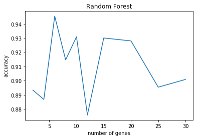
best_n, scores = search_gene(RFclf)
N=2 accuracy: 0.86 (+/- 0.12)
N=4 accuracy: 0.93 (+/- 0.14)
N=6 accuracy: 0.89 (+/- 0.17)
N=8 accuracy: 0.94 (+/- 0.16)
N=10 accuracy: 0.91 (+/- 0.13)
N=12 accuracy: 0.87 (+/- 0.26)
N=15 accuracy: 0.92 (+/- 0.14)
N=20 accuracy: 0.89 (+/- 0.10)
N=25 accuracy: 0.90 (+/- 0.11)
N=30 accuracy: 0.87 (+/- 0.09)
params = {
    'n_estimators': [100, 150, 300],
    'max_depth' : [30, 60, 90, None],
    'class_weight' : ['balanced']
}

search_param(RFclf, params, best_n)
N=8:
Best Params: {'class_weight': 'balanced', 'max_depth': 90, 'n_estimators': 150}

0.95 (+/-0.1) for {'class_weight': 'balanced', 'max_depth': 30, 'n_estimators': 100}
0.95 (+/-0.15) for {'class_weight': 'balanced', 'max_depth': 30, 'n_estimators': 150}
0.97 (+/-0.07) for {'class_weight': 'balanced', 'max_depth': 30, 'n_estimators': 300}
0.96 (+/-0.1) for {'class_weight': 'balanced', 'max_depth': 60, 'n_estimators': 100}
0.97 (+/-0.07) for {'class_weight': 'balanced', 'max_depth': 60, 'n_estimators': 150}
0.97 (+/-0.07) for {'class_weight': 'balanced', 'max_depth': 60, 'n_estimators': 300}
0.95 (+/-0.1) for {'class_weight': 'balanced', 'max_depth': 90, 'n_estimators': 100}
0.98 (+/-0.06) for {'class_weight': 'balanced', 'max_depth': 90, 'n_estimators': 150}
0.97 (+/-0.07) for {'class_weight': 'balanced', 'max_depth': 90, 'n_estimators': 300}
0.92 (+/-0.18) for {'class_weight': 'balanced', 'max_depth': None, 'n_estimators': 100}
0.95 (+/-0.15) for {'class_weight': 'balanced', 'max_depth': None, 'n_estimators': 150}
0.96 (+/-0.1) for {'class_weight': 'balanced', 'max_depth': None, 'n_estimators': 300}
Use the gene names from best train gene set and extract the data corresponding to these genes from the test set. Convert test set to “gene-in-columns” format to prepare it for classification.
best_n = 8
y_test = test_data.loc[pd.read_csv('pp5i_train.top'+str(best_n)+'.gr.csv').drop(labels='Class',
                                                                           axis=1).columns.tolist(), :].T.reset_index(drop=True)
Generate predictions for the test set
Now have the best train file, pp5i_train.bestN.csv, (with 69 samples and bestN number of genes found) and a corresponding test file, pp5i_test.bestN.csv, with the same genes and 23 test samples.
pd.read_csv('pp5i_train.top'+str(best_n)+'.gr.csv').to_csv('pp5i_train.best'+str(best_n)+'.csv', index=False)
y_test.to_csv('pp5i_test.best'+str(best_n)+'.csv', index=False)
Use the best train file and the matching test file and generate predictions for the test file class.
from sklearn.metrics import classification_report
from sklearn.utils import class_weight

x_train = pd.read_csv('pp5i_train.best'+str(best_n)+'.csv').drop(labels='Class', axis=1).values.tolist()
y_train = LE.transform(np.ravel(pd.read_csv('pp5i_train.best'+str(best_n)+'.csv', usecols=['Class']).values.tolist()))
sample_weight = class_weight.compute_sample_weight('balanced', y_train)

clf = RandomForestClassifier(n_estimators=150, max_depth=90, n_jobs=-1, class_weight='balanced')
clf.fit(x_train, y_train, sample_weight=sample_weight)
np.savetxt('pp5i_test_class.txt', LE.inverse_transform(clf.predict(y_test)), fmt='%s')
print(classification_report(y_train, clf.predict(x_train), target_names=classes))
precision    recall  f1-score   support

         EPD       1.00      1.00      1.00        10
         JPA       1.00      1.00      1.00         6
         MED       1.00      1.00      1.00        39
         MGL       1.00      1.00      1.00         7
         RHB       1.00      1.00      1.00         7

   micro avg       1.00      1.00      1.00        69
   macro avg       1.00      1.00      1.00        69
weighted avg       1.00      1.00      1.00        69