BOLD fMRI
Motivation
Blood oxygen level dependent functional magnetic resonance imaging (BOLD fMRI) is the most common method for measuring human brain activity non-invasively in-vivo. BOLD fMRI images are 4-dimensional, consisting of a time series of 3d volume, acquired in quick succession (every 1 or 2 seconds) typically over a period of 8 — 15 minutes.
Here, we will work with “multisubject, multimodal face processing” dataset (subject-01) available at openneuro.org. This dataset involves presentation of images of faces to the subject while acquiring BOLD fMRI images of the subject’s brain activity. Here, we will preprocess these scans and then, localize the brain area that processes faces.
Preparation
We need both afni and FSL software packages. Install VirtualBox and then download Neurodebian and open it in VirtualBox by selecting File->Import Appliance. Neurodebian is a Linux distribution of the Debian flavor.
Once installed, we will be able to run the preprocessing pipeline on the data from openneuro.
Basic pre-preprocessing
Basic preprocessing includes motion correction, bandpass filtering, spatial smoothing. Run pre-processing pipeline pipeline.sh from the command terminal. The pipeline will take roughly 5 — 10 minutes to run, depending on hardware setup. The processing pipeline will produce a final output called clean_bold.nii.gz, we will use this image for further work.
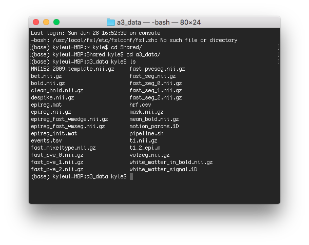
Above is a screenshot of the directory after running pipeline.sh.
Localize task activation
Briefly, task-based analysis procedure is as follows:
- Clean the BOLD images (using pipeline.sh);
- Load the clean_bold.nii.gz image output by pipeline.sh and events.tsv which corresponding to each BOLD image;
- Using the timing form events.tsv, create an “ideal time series” that represents how the brain should react to the stimulus (face=1, no face=0);
import nibabel as nib
import pandas as pd
import numpy as np
import matplotlib.pyplot as plt

clean_bold = nib.load('/clean_bold.nii.gz')
events = pd.read_csv('/events.tsv', delimiter='\t')
tr = clean_bold.header.get_zooms()[3]

ts = np.zeros(int(tr * clean_bold.shape[3]))

ts[np.round(events[~events['stim_type'].isna()]['onset'].values).astype('uint16')] = 1

plt.plot(ts); plt.xlabel('time(seconds)');

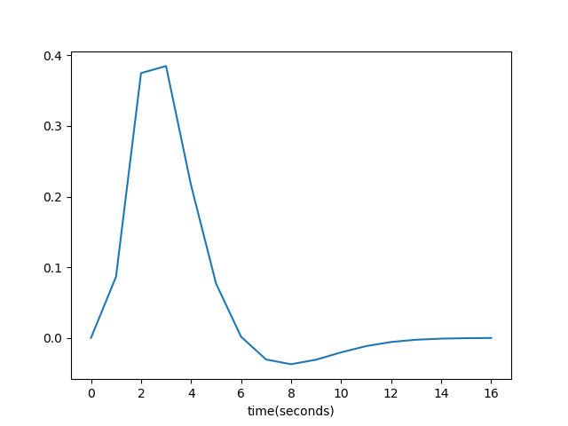
- Convolve the “ideal time series” the hemodynamic response function (HRF), we can use pandas load hrf.csv
hrf = pd.read_csv('hrf.csv', header=None);hrf = pd.read_csv('hrf.csv', header=None).values.ravel() plt.plot(hrf); plt.xlabel('time(seconds)');
import scipy.signal as signal

conved = signal.convolve(ts, hrf, mode='full')[:ts.shape[0]]

plt.plot(ts); plt.plot(conved*3); plt.xlabel('time(seconds)');

- Correlate the convolved ideal with the BOLD signal in each voxel;
conved = conved[::int(tr)]
img = clean_bold.get_fdata()

meansub_img = img - np.expand_dims(img.mean(-1), 3)
meansub_conved = conved - conved.mean()

corrs = (meansub_img * meansub_conved).sum(-1) / \
    np.sqrt((meansub_img * meansub_img).sum(-1)) / np.sqrt(np.dot(meansub_conved, meansub_conved))

corrs[np.isnan(corrs)] = 0
from sklearn.metrics import mutual_info_score

def MI(a):
    c_xy = np.histogram2d(a, conved)[0]
    return mutual_info_score(None, None, contingency=c_xy)

mi = np.apply_along_axis(MI, 3, img)
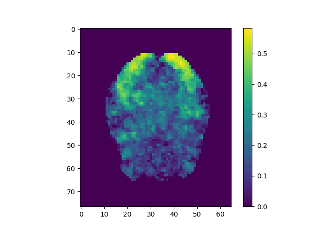
- Visualize the correlation map to see where in the brain the activation is strongest.
plt.imshow(np.rot90(corrs.max(2))); plt.colorbar();
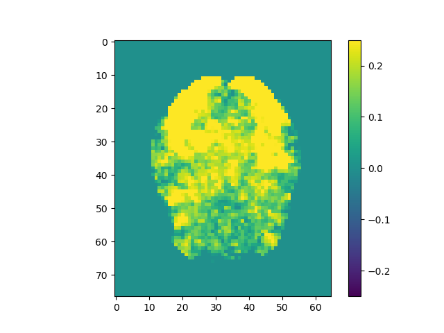
plt.imshow(np.rot90(corrs.max(2)), vmin=-0.25, vmax=0.25); plt.colorbar();
plt.imshow(np.rot90(mi.max(2))); plt.colorbar();
plt.imshow(np.rot90(mi.max(2)), vmin=-0.25, vmax=0.25); plt.colorbar();
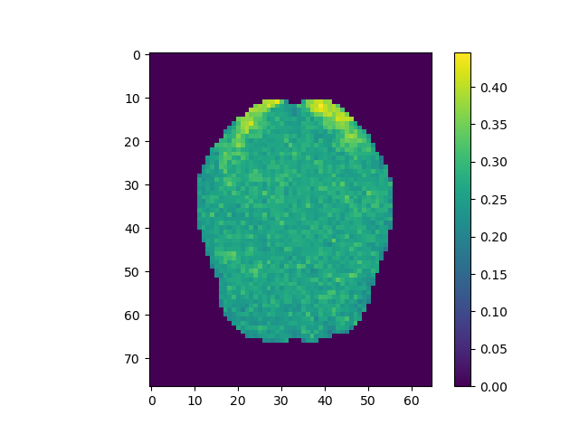
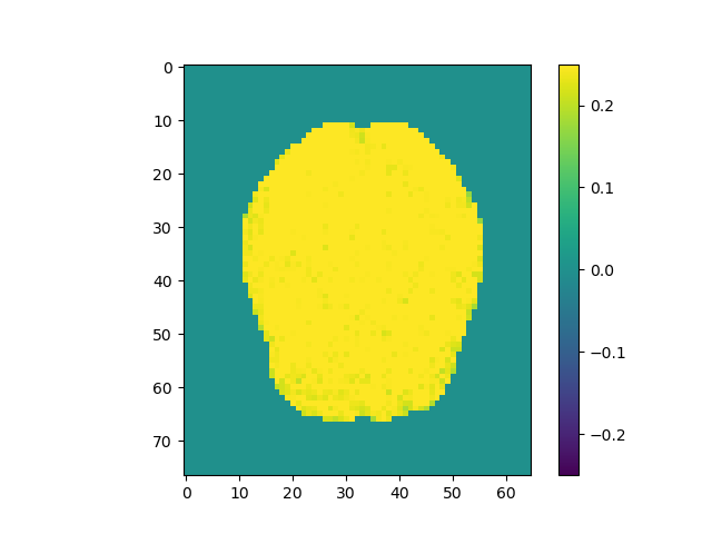
Use the above steps, we find the brain area which correlates to viewing of faces. We displayed a figure with maximum z-slice among 46 slices and a final activation map using imshow with vmin=-0.25 and vmax=0.25. There are some clusters near the back of the brain with high correlation values.
No pre-processing
Repeat the above, but leave out step 1 (use bold.nii.gz, without pre-processing, instead of the clean_bold.nii.gz output by pipeline.sh):
raw = nib.load('bold.nii.gz').get_fdata()

meansub_raw = raw - np.expand_dims(raw.mean(-1), 3)

corrs_raw = (meansub_raw * meansub_conved).sum(-1) / \
    np.sqrt((meansub_raw * meansub_raw).sum(-1)) / np.sqrt(np.dot(meansub_conved, meansub_conved))

corrs_raw[np.isnan(corrs_raw)] = 0
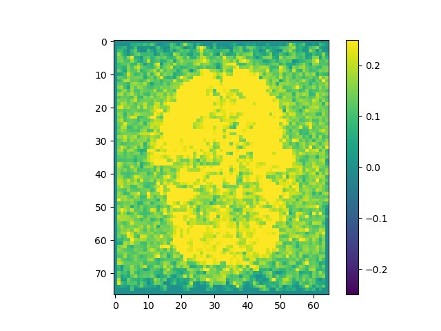
plt.imshow(np.rot90(corrs_raw.max(2))); plt.colorbar();
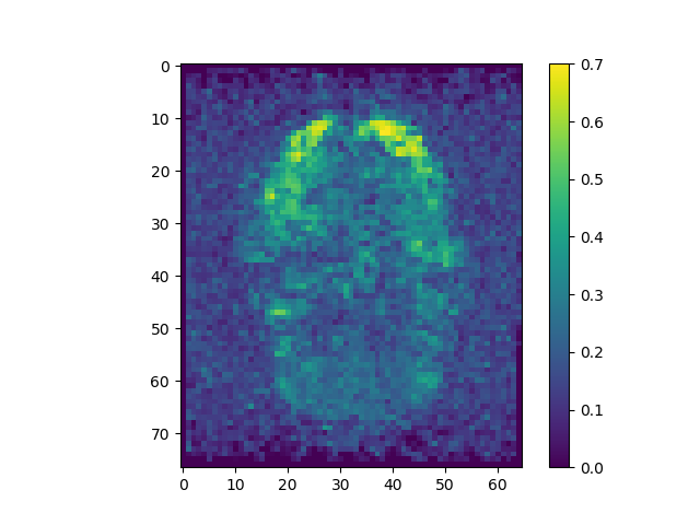
plt.imshow(np.rot90(corrs_raw.max(2)), vmin=-0.25, vmax=0.25); plt.colorbar();
mi_raw = np.apply_along_axis(MI, 3, raw)

plt.imshow(np.rot90(mi_raw.max(2))); plt.colorbar();
plt.imshow(np.rot90(mi_raw.max(2)), vmin=-0.25, vmax=0.25); plt.colorbar();
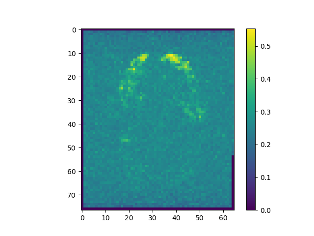
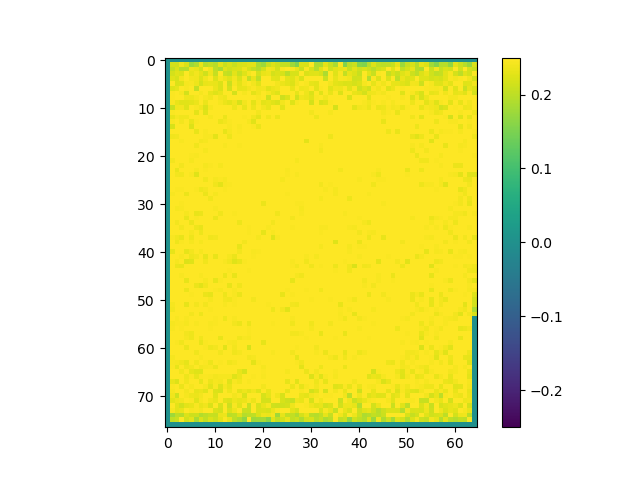
The correlations are stronger when pre-processing is included.
Multi-subject analysis
The dataset on openneuro contains scans from 16 subjects. In previous part, we only processed data from sub-01. Each subject actually contains multiple BOLD fMRI runs, here we just use T1 and first fMRI from all 16 subjects. However, we may use all the BOLD scans from each subject and average the resulting correlation maps to produce a more clear correlation.
Batch processing
Once we have all subjects, create a separate folder for each subject and place each subjects’ data in their own separate folder. Then, run the pre-processing pipeline on each subject separately (this may take up to 1 hour). We can simply place the script in each subject’s folder and run it as-is at the command line, or create a for loop surrounding the pre-processing code in the pipeline.sh file to loop over all subjects automatically.
Once each subject has been pre-processed, run the correlation analysis as in previous part on each subject and save the output as a .nii file into the same subject’s directory. Be sure to keep the same header transform as the input image when saving using nibabel, otherwise the correlation map will not be in the same space (see below):
corrs_nifti = nib.Nifti1Image(corrs, clean_bold.affine)
nib.save(corrs_nifti, 'corrs.nii.gz')

mi_nifti = nib.Nifti1Image(mi, clean_bold.affine)
nib.save(mi_nifti, path+str(i)+'/mi.nii.gz')
Using epireg.mat, bring the correlation map into the subject’s T1 space (see below):
flirt -in corrs.nii.gz -ref t1.nii.gz -applyxfm -init epireg.mat -out corrs_in_t1.nii.gz
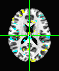
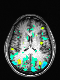
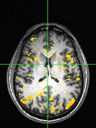
Visualize the correlation map as an overlay on the T1 using afni. Increase the threshold to find the brain area of maximum activation, and show each subject’s correlation map overlayed on the T1 in afni with a threshold of 0.15. Here we just show one image with sub-01 correlation map overlayed on the T1 (axial view) as well as for mutual information:
Group average
Once we have obtained each subjects correlation map in their native T1 space, the last step is to bring all subjects into the same space and average the correlation map, to create a ‘grand average’ of where the brain processes faces. We can use “template brain” MNI152_2009_template.nii.gz. Using flirt or ANTs, register each subject’s skull-stripped T1 to this template image and save the transform. Then, apply the tranform to the correlation map in T1 space, bringing each subjects’ correlation map into template space. Finally, once all subjects’ correlation maps have been aligned to the “template brain”, average them, creating a “grand average” correlation map.
corrs_nifti = nib.load('1/corrs_in_template.nii.gz')
corrs = corrs_nifti.get_fdata()
for i in range(2, 17):
    corrs += nib.load(str(i)+'/corrs_in_template.nii.gz').get_fdata()

corrs /= 16
corrs_nifti = nib.Nifti1Image(corrs, corrs_nifti.affine)
nib.save(corrs_nifti, 'corrs_in_template.nii.gz')

mi_nifti = nib.load('1/mi_in_template.nii.gz')
mi = mi_nifti.get_fdata()
for i in range(2, 17):
    mi += nib.load(str(i)+'/mi_in_template.nii.gz').get_fdata()

mi /= 16
mi_nifti = nib.Nifti1Image(mi, mi_nifti.affine)
nib.save(mi_nifti, 'mi_in_template.nii.gz')
Display this grand average correlation map as an overlay on the “template brain” in afni, with a suitable threshold, showing the region of maximum correlation.
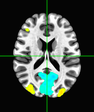
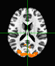
Some faces may result in higher BOLD activation than others. Using events.tsv, and the knowledge that the hemodynamic response is roughly 4.5 seconds after the onset of the face, locate the area in the brain that distinguishes famous faces and unfamiliar faces. This can be done by isolating all BOLD time points 4.5 seconds after the onset of a famous face (F1) and also isolating all BOLD time points 4.5 seconds after onset of unfamiliar face (F2) and then performing a t-test (F1-F2) which will then give a t-value and a p-value in each voxel showing which voxel had significant differences in their response from famous to unfamiliar faces. Show this grand average t-map overlayed on the template brain.
import scipy.stats as stats

for i in range(1, 17):
    clean_bold = nib.load(str(i)+'/clean_bold.nii.gz')
    img = clean_bold.get_fdata()
    tr = clean_bold.header.get_zooms()[-1]
    events = pd.read_csv(str(i)+'/events.tsv', delimiter='\t')
    f1id = np.round((events['onset'][events['stim_type'] != 'FAMOUS'].values+4.5)/tr).astype('uint16')
    f2id = np.round((events['onset'][events['stim_type'] != 'UNFAMILIAR'].values+4.5)/tr).astype('uint16')
    f1 = img[:, :, :, f1id]
    f2 = img[:, :, :, f2id]
    tmap = stats.ttest_ind(f1, f2, axis=3)[0]
    tmap_nifti = nib.Nifti1Image(tmap, clean_bold.affine)
    nib.save(tmap_nifti, str(i)+'/tmap.nii.gz')


tmap_nifti = nib.load('1/tmap_in_template.nii.gz')
tmap = tmap_nifti.get_fdata()
for i in range(2, 17):
    tmap += nib.load(str(i)+'/tmap_in_template.nii.gz').get_fdata()

tmap /= 16
tmap_nifti = nib.Nifti1Image(tmap, tmap_nifti.affine)
nib.save(tmap_nifti, 'tmap_in_template.nii.gz')
