Logistic Regression and Application (R)

Logistic Regression and Classification

Logistic regression is a machine learning classification algorithm used to assign observations to a discrete set of classes. Some of the well known examples of this kind of classification are email spam or ham, transactions fraud, tumor malignant or benign. Given a feature vector $X$ and a qualitative response $Y$ taking values in the set $C = {C_{1}, \dots, C_{k}}$ , a classification task is to build a function $f : X \to Y$ (classifier) that takes the feature vector $X$ as input and predicts the value for $Y$ , i.e. $Y \in C$ . The model or function or classifier $f$ is built using a set of training observations $(x_{1}, y_{1}), \dots, (x_{n}, y_{n})$ for a given $n$ . In order to avoid crisp decisions and give to the user flexibility in the classification process, often we are more interested in estimating the probabilities that $Y$ belongs to each category in $C$ than estimating directly the value of $Y$ .

Unlike linear regression where the target variable $y$ is related to the features via the linear relationship:

y = β_{0} + β_{1} x_{1} + \dots + β_{k} x_{k} + ϵ,

in logistic regression, we relate $p (y)$ , the probability of $Y$ belonging to a certain class (which ranges between 0 and 1), to the features $x_{1}, \dots, x_{k}$ via the logistic (or logit) transformation given by

\log \frac{p (y)}{1 - p (y)} = β_{0} + β_{1} x_{1} + \dots + β_{k} x_{k} .

Define $S (w)$ as the logistic sigmoid function give by

S (w) = \frac{1}{1 + e^{- w}}

Display a graph of $S (w)$ for $- \infty < w < \infty$

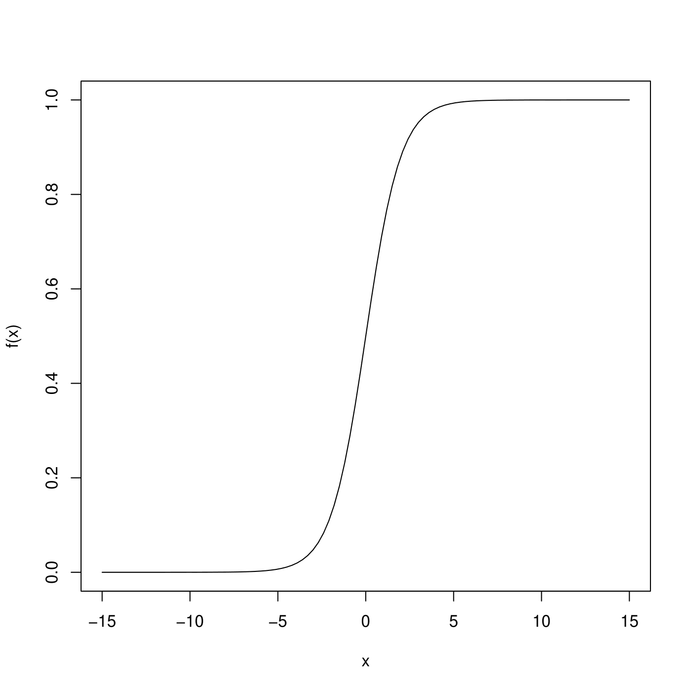
it shows no matter what values $β_{0}, β_{1}, \dots, β_{k}$ or $x_{1}, \dots, x_{k}$ take, $p (y)$ will always have values between 0 and 1.

To summarize, the logistic regression starts with the idea of linear regression and transforms its output using the sigmoid function to return a probability value.

Maximum Likelihood Estimation (MLE) of the Model

In logistic regression, our goal is to learn a set of parameters $β^{T} = (β_{0}, β_{1}, \dots, β_{k})$ using the available estimation. Although we could use (non-linear) least squares to fit the logistic regression model, the more general method of maximum likelihood estimation (MLE) is preferred, since it has better statistical properties. The idea behind MLE is to choose the most likely values of the parameters $β_{0}, \dots, β_{n}$ given the observed sample

(x_{1}^{(i)}, \dots, x_{k}^{(i)}, y_{i}), 1 \leq i \leq n .

In logistic regression, the probability model is based on the binomial distributions:

f (x_{i}, p_{i}) = f (y_{i}, p_{i}) = {\begin{cases} p_{i} & if y_{i} = 1 \\ 1 - p_{i} & if y_{i} = 0, \end{cases}

where $x_{i} = (x_{1}^{(i)}, \dots, x_{k}^{(i)})^{T}$ is the vector of features and $0 < p_{i} < 1$ are the probabilities associated to the binomials in the model. In other words, the probability of the feature vector $x_{i}$ specifying the class $y_{i} = 1$ occurs with probability $p_{i}$ , that is

p (y_{i} = 1) = p_{i} = \frac{e^{β_{0} + β_{1} x_{1}^{(i)} + \dots + β_{k} x_{k}^{(i)}}}{1 + e^{β_{0} + β_{1} x_{1}^{(i)} + \dots + β_{k} x_{k}^{(i)}}} = \frac{e^{x_{i}^{T} β}}{1 + e^{x_{i}^{T} β}}

where $β = (β_{0}, β_{1}, \dots, β_{k})^{T}$ and $x_{i} = (1, x_{1}^{(i)}, \dots, x_{k}^{(i)})^{T}$ for $1 \leq i \leq n$ .

Typically, numerical approximations and optimization procedures are used to find the (best) vector $β^{*}$ satisfying

β^{*} = argmax (ℓ (β))

There are many known techniques and here I implement my own procedure which is a logistic regression classifier using gradient ascent as illustrated in the following algorithm.

    % gradient ascent algorithm
    \begin{algorithm}
    \caption{Algorithm for finding $\boldsymbol{\beta}^*$}
    \begin{algorithmic}
    \STATE Set $\eta\in [0, 1]$ (learning coefficient)
    \STATE Set $\epsilon > 0$ (tolerance term)
    \STATE $\boldsymbol{\beta}^{(0)}\leftarrow initial\_value$
    \FOR{$t = 0, 1, \cdots$}
        \STATE Compute the gradient: $g_t = \nabla\ell(\boldsymbol{\beta}^{(t)})$
        \STATE Update the coefficients: $\boldsymbol{\beta}^{(t+1)}\leftarrow \boldsymbol{\beta}^{(t)} + \eta g_t$
        \STATE Iterate until: $||\boldsymbol{\beta}^{(t+1)} - \boldsymbol{\beta}^{(t)}|| < \epsilon$.
    \ENDFOR
    \RETURN $\boldsymbol{\beta}^{(t^\text{final})}$ (final coefficients)
    \end{algorithmic}
    \end{algorithm}

Here I provide an implementation in the simple case where there is only one feature variable $x_{1}$ . I have uploaded the data set SAheart.data on GitHub, the task here is to predict the value of the variable chd (response, coronary heart disease diagnosis) from the feature value ldl (low density lipoprotein cholesterol). I use the first 100 rows for training and any values in the remaining rows for testing. Following procedures are identified:

Load and clean data.

# Load data
data <- read.csv('SAheart.data')
data <- data[, c('ldl','chd')]

# remove NA rows
data <- na.omit(data)

Normalize the feature variable $x_{1}$ (see Nota-Bene below).

# Normalize the feature variable
normalize <- function(x) { (x - mean(x)) / sd(x) }
data['ldl'] <- lapply(data['ldl'], normalize)

Split training data and test data.

# Train test split
train <- data[1:100, ]
test <- tail(data, -100)

X_train <- train$ldl
y_train <- train$chd
X_test <- test$ldl
y_test <- test$chd

Calculate objective function $ℓ (β_{0}, β_{1})$ .

# Sigmoid function
sigmoid <- function(w) { 1/(1+exp(-w)) }

# Objective Function
cost <- function(beta, X, y) {
    p <- sigmoid(X %*% beta)
    t(y)%*%log(p) + t(1-y)%*%log(1-p)
}

Calculate gradient function $\nabla ℓ (β_{0}, β_{1})$ .

# Gradient function
grad <- function(beta, X, y) {
    t(X) %*% (y - sigmoid(X%*%beta))
}

Create logistic regression and complete implementation of gradient ascent. It is much better to look ar the convergence of the values $ℓ (β_{0}, β_{1})$ than the convergence of the parameters themselves.

# Fit logistic regression, set learning coefficient and tolerance term
fit_logit <- function(X, y, bias=T, eta=10e-3, eps=10e-6, max_iters=200) {
    # Type conversion
    if (!is.matrix(X)) { X <- as.matrix(X) }
    if (!is.matrix(y)) { y <- as.matrix(y) }

    # Add bias
    if (bias) { X <- cbind(1, X) }

    # Algorithm initialization
    iters <- 0

    # Initialize beta to 0
    beta <- matrix(0, ncol(X))
    prev_cost <- cost(beta, X, y)

    # Update the beta using gradient ascent until converaged or reach max iterations
    while (iters < max_iters) {
        iters <- iters+1
        # Compute the gradient and update beta
        beta <- beta + eta*grad(beta, X, y)

        curr_cost <- cost(beta, X, y)
        # Check whether converaged
        if (abs(curr_cost-prev_cost) < eps) { break }

        prev_cost <- curr_cost
    }
    # Create the logit Object
    logit <- list(bias=bias)
    logit[['beta']] <- beta
    logit[['probs']] <- sigmoid(X%*%beta)
    logit[['residuals']] <- y - logit[['probs']]
    logit[['preds']] <- ifelse(logit[['probs']] > .5, 1, 0)
    logit[['score']] <- sum(logit[['preds']] == y)/nrow(y)
    logit[['iters']] <- iters
    attr(logit, 'class') <- 'logit'
    logit
}

Predict the labels for a set of test examples.

# Predict on new data
predict.logit <- function(logit, X, probs=F, ..) {
    if (!is.matrix(X)) { X <- as.matrix(X) }
    if (logit[['bias']]) { X <- cbind(1, X) }
    if (probs) { sigmoid(X%*%logit[['beta']]) }
    else { ifelse(sigmoid(X%*%logit[['beta']]) > .5, 1, 0) }
}

Try different learning rate $η$ values.

# Score function
score <- function(y_pred, y) {
    if (!is.matrix(y_pred)) { y_pred <- as.matrix(y_pred) }
    if (!is.matrix(y)) { y <- as.matrix(y) }
    sum(y_pred == y)/nrow(y)
}

# Try different learning rate
etas <- list(.25, .2, .15, .1, .05, .01, .005)

for (eta in etas) {
    logit.fit <- fit_logit(X_train, y_train, eta=eta)
    # Predict the labels for test examples
    y_pred <- predict(logit.fit, X_test)
    # print accuracy score
    print(score(y_pred, y_test))
}

The output is

[1] 0.3314917
[1] 0.3259669
[1] 0.4585635
[1] 0.6657459
[1] 0.6823204
[1] 0.6823204
[1] 0.6823204

References

Nota-Bene

In machine learning, it is a standard routine to normalize or scale the feature variables to speed up the convergence of the learning algorithms and to ensure that the features contribute equally to the learning task. One way to achieve the normalization if by making the values of each feature in the data have zero mean (when subtracting the mean in the numerator) and unit variance, i.e., replace the variable $x_{1}$ with $\frac{x_{1} - μ}{σ}$ , where $μ$ and $σ$ are respectively the mean and the standard deviation of the values of $x_{1}$ in the training data.